In MATLAB, all data is stored in the form of arrays or matrices. This section mainly introduces methods for constructing arrays and matrices.
Note: Arrays and matrices belong to the category of data structures, not data types. Please distinguish them conceptually.
Arrays
Constructing an array in MATLAB is very simple; you just need to separate the array elements with spaces or commas and enclose them in square brackets. For example:
x=[0 2 3 6 7 8]constructs an array x with 6 elements.
In addition to direct construction, there are some commonly used construction methods. Two of them are introduced below: the increment method and the linspace function method.
1. Constructing Arrays Using the Increment Method
Using the colon operator (first:last) provided by MATLAB can generate a 1×n matrix, i.e., an array. The elements in the array are sequentially from first to last. By default, the sequence is generated with an increment of 1, meaning the number behind is 1 larger than the number immediately preceding it.
[Example 2-7] Enter in the Command Window:
A = 10:15
A =
    10    11    12    13    14    15
Arrays do not have to consist of positive integers; they can also include negative values and decimals. Such as:
A = -2.5:2.5
A =
   -2.5000   -1.5000   -0.5000    0.5000    1.5000    2.5000
By default, when MATLAB creates a sequence, the increment is always 1, even if the last value is not an integer. Such as:
A = 1:6.3
A =
     1     2     3     4     5     6
Similarly, sequences generated by the colon operator are always in ascending order (not descending order). The following attempt to generate a descending numerical sequence fails.
A = 9:1
A =
   Empty matrix: 1-by-0
In fact, you can specify the increment step value when using the colon operator. You can use the format (first:step:last). For example, create a numerical sequence from 10 to 50 with an increment of 5:
A = 10:5:50
A =
    10    15    20    25    30    35    40    45    50
The increment can also be a decimal. For example, in the following example, the increment is 0.2:
A = 3:0.2:3.8
A =
    3.0000    3.2000    3.4000    3.6000    3.8000
When a negative increment is specified, a descending numerical sequence is created:
A = 9:-1:1
A =
     9     8     7     6     5     4     3     2     1
2. Constructing Arrays Using the linspace Function Method
To construct an array using the linspace function method, you need to specify the first and last values and the total number of elements. Its basic form is:
x=linspace(first,last,num)Where first, last, and num are the first element, last element, and number of elements of the x array, respectively.
[Example 2-8] Enter in the Command Window:
x=linspace(0,10,5)
x =
     0    2.5000    5.0000    7.5000   10.0000
Matrices
In MATLAB, two-dimensional arrays are called matrices. Several methods for creating matrices are introduced below.
1. Simple Creation Method
The simplest way to create a matrix in MATLAB is to use the matrix creation symbol []. Entering multiple elements within square brackets creates a row of a matrix. Separate each element with a comma or a space:
row = [E1, E2, ..., Em] row = [E1 E2 ... Em][Example 2-9] Enter the following code to create a row containing 5 elements:
A = [12 62 93 -8 22];If you want to start a new line, you can use a semicolon to terminate the current line:
A = [row1; row2; ...; rown]Below, create a numerical matrix with 3 rows and 5 columns. Note that all rows must have the same number of elements:
A = [12 62 93 -8 22; 16 2 87 43 91; -4 17 -72 95 6]
A =
    12    62    93    -8    22
    16     2    87    43    91
    -4    17   -72    95     6
2. Constructing Special Matrices
MATLAB provides several functions for creating different matrices, as shown in Table 2-4. Using these functions, you can construct various special matrices.
Table 2-4: Functions for Constructing Special Matrices
| Function | Description |
|---|---|
| ones | Create a matrix where all elements are 1. |
| zeros | Create a matrix where all elements are 0. |
| eye | Create a matrix with 1s on the diagonal and 0s elsewhere. |
| accumarray | Distribute elements of an input matrix to specified locations in an output matrix. |
| diag | Create a diagonal matrix based on a vector. |
| magic | Create a square matrix where the sum of rows, columns, and diagonals are equal. |
| rand | Create a matrix or array where elements are uniformly distributed random numbers. |
| randn | Create a matrix or array where elements are normally distributed random numbers. |
| randperm | Create a vector (1×n matrix) of random permutations. |
Most of the functions listed in Table 2-4 return matrices of double type. In addition, you can easily generate basic arrays of any numeric type using the ones, zeros, and eye functions.
To do this, you need to pass the MATLAB data type name as the last variable.
[Example 2-10] Enter in the Command Window:
A = zeros(4, 6, 'uint32')
A =
     0        0        0        0        0        0
     0        0        0        0        0        0
     0        0        0        0        0        0
     0        0        0        0        0        0
[Example 2-11] Create a 5×5 magic square matrix below:
A = magic(5)
A =
    17    24     1     8    15
    23     5     7    14    16
     4     6    13    20    22
    10    12    19    21     3
    11    18    25     2     9
Note: The sum of the numbers in each row, each column, and each main diagonal in the matrix equals 65.
[Example 2-12] Create a matrix or array of elements that are random numbers with a uniform distribution below, multiplying each element by 20:
A = rand(5) * 20
A =
    3.8686   13.9580    9.9310   13.2046   14.5423
   13.6445    7.5675   17.9954    6.8394    6.1858
    6.0553   17.2002   16.4326    5.7945   16.7699
   10.8335   17.0731   12.8982    6.8239   11.3614
    3.0175   11.8713   16.3595   10.6816    7.4083
[Example 2-13] Create a diagonal matrix based on vector elements below. You can place vector elements on the main diagonal of the matrix, or above or below the main diagonal, as shown below, where -1 means placing the vector elements below the main diagonal:
A = [12 62 93 -8 22];
B = diag(A, -1)
B =
     0     0     0     0     0     0
    12     0     0     0     0     0
     0    62     0     0     0     0
     0     0    93     0     0     0
     0     0     0    -8     0     0
     0     0     0     0    22     0
3. Concatenating Matrices
Matrix concatenation is the formation of a new matrix by joining one or more matrices together. The symbol [] is not only a matrix constructor but also the MATLAB concatenation operator. The expression C=[A B] concatenates matrices A and B horizontally, and the expression C=[A;B] concatenates them vertically.
[Example 2-14] Construct a new matrix C by concatenating matrices A and B vertically:
A = ones(2, 5) * 6;        % 2x5 matrix with elements 6
B = rand(3, 5);           % 3x5 matrix with random numbers
C = [A; B]              % Concatenate A and B vertically
C =
    6.0000    6.0000    6.0000    6.0000    6.0000
    6.0000    6.0000    6.0000    6.0000    6.0000
    0.6154    0.7382    0.9355    0.8936    0.8132
    0.7919    0.1763    0.9169    0.0579    0.0099
    0.9218    0.4057    0.4103    0.3529    0.1389
You can use concatenation to create matrices or even multidimensional arrays, but you cannot generate irregular shapes (they must be rectangular). If generating a matrix horizontally, each sub-matrix must have the same number of rows; if generating a matrix vertically, each sub-matrix must have the same number of columns.
Figure 2-2 shows two matrices of the same height combining horizontally into a new matrix.

Figure 2-2: Concatenating Matrices of the Same Height
Figure 2-3 shows the situation of horizontally combining two matrices of different heights. However, MATLAB does not allow this.
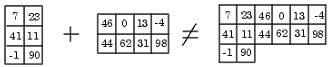
Figure 2-3: Concatenating Matrices of Different Heights
Use the functions shown in Table 2-5 to combine multiple matrices into a new matrix.
Table 2-5: Functions for Concatenating Matrices
| Function | Description |
|---|---|
| cat | Concatenate matrices along a specified dimension. |
| horzcat | Concatenate matrices horizontally. |
| vertcat | Concatenate matrices vertically. |
| repmat | Create a new matrix by replicating and tiling a matrix. |
| blkdiag | Create a block diagonal matrix using existing matrices. |
The following examples demonstrate the use of the functions in Table 2-5.
Using the cat, horzcat, and vertcat functions can replace the [] symbol to achieve matrix concatenation.
[Example 2-15] The following two statements can achieve the effect of the command C=[A;B]:
C = cat(1, A, B);       % Concatenate along the first dimension
C = vertcat(A, B);      % Concatenate vertically
The repmat function can create a matrix using multiple copies of an existing matrix. The command repmat(M, v, h) replicates matrix M vertically v times and horizontally h times.
[Example 2-16] Copy the existing matrix A into the new matrix B below.
A = [8 1 6; 3 5 7; 4 9 2]
A =
     8     1     6
     3     5     7
     4     9     2
B = repmat(A, 2, 4)
B =
     8     1     6     8     1     6     8     1     6     8     1     6
     3     5     7     3     5     7     3     5     7     3     5     7
     4     9     2     4     9     2     4     9     2     4     9     2
     8     1     6     8     1     6     8     1     6     8     1     6
     3     5     7     3     5     7     3     5     7     3     5     7
     4     9     2     4     9     2     4     9     2     4     9     2
[Example 2-17] Use the blkdiag function to create a block diagonal matrix below.
A = magic(3);
B = [-9 -4 -2];
C = eye(2) * 8;
D = blkdiag(A, B, C)
D =
     8     1     6     0     0     0     0     0
     3     5     7     0     0     0     0     0
     4     9     2     0     0     0     0     0
     0     0     0    -9     0     0     0     0
     0     0     0    -4     0     0     0     0
     0     0     0    -2     0     0     0     0
     0     0     0     0     0     0     8     0
     0     0     0     0     0     0     0     8
4. Combining Different Types of Data
When concatenating matrices, if the matrices have different data types, MATLAB will automatically perform type conversion on some elements, and the resulting matrix will have the same type.
When concatenating a high-precision matrix with a low-precision matrix, the new matrix is of the low-precision type. For example, when concatenating single and double matrices, a single matrix is always generated. MATLAB will first convert the double elements to single.
[Example 2-18] If an empty matrix participates in matrix concatenation, the empty matrix will be ignored:
A = [5.36; 7.01; []; 9.44]
A =
    5.3600
    7.0100
    9.4400
[Example 2-19] Here are several examples of concatenating matrices of different types.
Concatenating single and double matrices
x = [single(4.5) single(-2.8) pi 5.73*10^300]
x =
    4.5000   -2.8000    3.1416       Inf
class(x)              % Display data type of x
ans =
single
Concatenating integer and double matrices
x = [int8(21) int8(-22) int8(23) pi 45/6]
x =
   21   -22    23     3     8
class(x)
ans =
int8
Concatenating character and double matrices
x = ['A' 'B' 'C' 68 69 70]
x =
ABCDEF
class(x)
ans =
char
Concatenating logical and double matrices
x = [true false false pi sqrt(7)]
x =
    1.0000         0         0    3.1416    2.6458
class(x)
ans =
double
5. Accessing Elements of a Matrix
You can access elements of a MATLAB matrix using indices and indexing.
To refer to specific elements in a matrix, you can specify its row number and column number using the following syntax, where A is the matrix variable. Specify in the order of row first, then column.
A(row, column)[Example 2-20] Access elements in a matrix below.
For the 4×4 magic square matrix A:
A = magic(4)
A =
    16     2     3    13
     5    11    10     8
     9     7     6    12
     4    14    15     1
Access the element at row 4, column 2 below:
A(4, 2)
ans =
    14
In MATLAB, you can reference elements in a matrix using a single index. When MATLAB stores data in a matrix, it is not saved in the shape displayed in the MATLAB Command Window, but as a single column of elements. This column of elements is composed of all columns in the matrix, with the elements of the next column added to the end of the previous column's elements in order. So, for matrix A:
A = [2 6 9; 4 2 8; 3 0 1]
A =
     2     6     9
     4     2     8
     3     5     1
It is saved in memory as the following sequence:
2, 4, 3, 6, 2, 5, 9, 8, 1
The element at row 3, column 2 in matrix A can be viewed as the 6th element in the actual saved sequence. To access this element, you can use the standard syntax A(3,2) or use A(6). When using linear indexing, if the matrix size is [d1 d2], i.e., d1 rows and d2 columns, the position of the element at (i,j) in the saved sequence is:
(j-1) * d1 + i
For example, the size of matrix A above is [3 3], so the position of the element at (3,2) in the saved sequence is (2-1)*3+3, which is 6.
If you know the row-column index but want to use linear indexing, you can use the sub2ind function to convert.
[Example 2-21] Convert the row-column index (3,2) of matrix A above to linear index 6:
A = [2 6 9; 4 2 8; 3 0 1];
linearindex = sub2ind(size(A), 3, 2)
linearindex =
     6
Similarly, use the ind2sub function to get the row-column index value based on the linear index value.
[Example 2-22] Enter in the Command Window:
[row col] = ind2sub(size(A), 6)
row =
     3
col =
     2
[Example 2-23] Suppose A is a 4×4 matrix. Use the row-column indexing method to find the sum of the elements in the 4th column below.
A = magic(4);
A(1,4) + A(2,4) + A(3,4) + A(4,4)
You can use the colon operator and the sum function to get the result of the second statement above:
sum(A(1:4,4))[Example 2-24] Change the values at every other element in matrix B to -10 below.
B = A;
B(1:3:16) = -10
B =
   -10     2     3   -10
     5    11   -10     8
     9   -10     6    12
   -10    14    15   -10
Using the end keyword can specify the last element of a certain dimension of a matrix. This method is suitable when you don't know how many rows or columns the matrix has. For example, you can use the following statement to replace values:
B(1:3:end) = -10Using a colon can reference all elements of a row or column of a matrix. Using the following statement, you can calculate the sum of all elements in the 2nd column of the 4×4 magic square matrix A.
sum(A(:, 2))
ans =
    34
Using a colon as a linear index can reference all elements in the entire matrix. The following statement displays all elements in matrix A and returns them in column order.
A(:)
ans =
    16
     5
     9
     4
     ...
    12
     1
6. Getting Information About Matrices
The functions in Table 2-6 can return information about the shape and size of a matrix.
Table 2-6: Functions Returning Matrix Information
| Function | Function |
|---|---|
| length | Returns the length of the longest dimension. |
| ndims | Returns the number of dimensions. |
| numel | Returns the number of elements. |
| size | Returns the length of each dimension. |
[Example 2-25] Demonstrate the application of some functions from Table 2-6 below.
A = rand(5) * 10;
A(4:5, :) = []
A =
    9.5013    7.6210    6.1543    4.0571    0.5789
    2.3114    4.5647    7.9194    9.3547    3.5287
    6.0684    0.1850    9.2181    9.1690    8.1317
% Calculate the mean of all element values in matrix A
sum(A(:))/numel(A)
ans =
    5.8909
% Find elements in the matrix with values between 5 and 7
if ndims(A) ~= 2
    return
end
[rows cols] = size(A);
for m = 1:rows
    for n = 1:cols
        x = A(m, n);
        if x >= 5 && x <= 7
            disp(sprintf('A(%d, %d) = %5.2f', m, n, A(m,n)))
        end
    end
end
Returns:
A(1, 3) = 6.15
A(3, 1) = 6.07
Note: Flow control statements are used here. For a detailed description of flow control, please refer to Chapter 3.
The functions in Table 2-7 are used to check whether elements in a matrix belong to a specified data type.
Table 2-7: Functions for Checking Data Types
| Function | Function |
|---|---|
| isa | Determine if input data belongs to a given type. |
| iscell | Determine if input data belongs to a cell array. |
| iscellstr | Determine if input data belongs to a string cell array. |
| ischar | Determine if input data belongs to a string. |
| isfloat | Determine if input data belongs to a floating-point array. |
| isinteger | Determine if input data belongs to an integer array. |
| islogical | Determine if input data belongs to a logical array. |
| isnumeric | Determine if input data belongs to a numeric array. |
| isreal | Determine if input data belongs to a real-valued array. |
| isstruct | Determine if input data belongs to a structure array. |
[Example 2-26] Find numeric elements from a vector.
A = [5+7i 8/7 4.23 39j pi 9-2i];
for m = 1:numel(A)
    if isnumeric(A(m)) && isreal(A(m))
        disp(A(m))
    end
end
Return values:
1.1429
4.2300
3.1416
The functions in Table 2-8 can check whether elements in a matrix are of a specified data structure.
Table 2-8: Functions for Checking Data Structures
| Function | Function |
|---|---|
| isempty | Determine if input data is empty. |
| isscalar | Determine if input data is a scalar. |
| issparse | Determine if input data is a sparse matrix. |
| isvector | Determine if input data is a vector. |
Multidimensional Arrays
You can create multidimensional arrays in the same way you create two-dimensional matrices. In addition, MATLAB provides a special concatenation function for generating multidimensional arrays.
1. Generating Multidimensional Arrays Using Indexing
One way to create a multidimensional array is to first create a 2D array and then extend it.
[Example 2-27] Generate a multidimensional array using indexing.
Enter in the Command Window:
A = [5 7 8; 0 1 9; 4 3 6];A is a 3×3 numeric array, meaning its row dimension and column dimension are both 3. Add a third dimension to A.
A(:,:,2) = [1 0 4; 3 5 6; 9 8 7]You can expand a multidimensional array by increasing its index values, for example:
A(:,:,3) = 5;
A(:,:,3)
ans =
     5     5     5
     5     5     5
     5     5     5
Now expand A into a 3×3×2 four-dimensional array. Enter:
A(:,:,1,2) = [1 2 3; 4 5 6; 7 8 9];
A(:,:,2,2) = [9 8 7; 6 5 4; 3 2 1];
A(:,:,3,2) = [1 0 1; 1 1 0; 0 1 1];
2. Generating Multidimensional Arrays Using MATLAB Functions
You can generate multidimensional arrays using the same methods as creating 2D arrays (such as using randn, ones, and zeros functions, etc.). Each variable provided represents the size of the corresponding dimension in the generated array.
[Example 2-28] Create a 4×3×2 array with normally distributed random numbers.
Enter in the Command Window:
B = randn(4,3,2)To generate an array where all elements are the same constant, use the repmat function.
[Example 2-29] E.g.:
B = repmat(5,[3 4 2])
B(:,:,1) =
     5     5     5     5
     5     5     5     5
     5     5     5     5
B(:,:,2) =
     5     5     5     5
     5     5     5     5
     5     5     5     5
Note: By setting any dimension of an array to an empty array, you can make the size of that dimension 0.
3. Generating Multidimensional Arrays Using the cat Function
The cat function is a simple way to create multidimensional arrays; it aggregates multiple arrays together along a specified dimension. Its syntax is:
matlab
B = cat(dim,A1,A2…)
Where A1, A2, etc., are the arrays to be concatenated, and dim is the dimension.
[Example 2-30] Create a new array B using the cat function below:
B = cat(3,[2 8; 0 5],[1 3; 7 9])
B(:,:,1) =
     2     8
     0     5
B(:,:,2) =
     1     3
     7     9
The cat function accepts any original data and new data. In addition, you can nest calls to the cat function.
[Example 2-31] Create a four-dimensional array below.
A = cat(3,[9 2; 6 5],[7 1; 8 4]);
B = cat(3,[3 5; 0 1],[5 6; 2 1]);
D = cat(4,A,B,cat(3,[1 2; 3 4],[4 3;2 1]))
D(:,:,1,1) =
     9     2
     6     5
D(:,:,2,1) =
     7     1
     8     4
D(:,:,1,2) =
     3     5
     0     1
D(:,:,2,2) =
     5     6
     2     1
D(:,:,1,3) =
     1     2
     3     4
D(:,:,2,3) =
     4     3
     2     1